Model Building
ParamRF provides a models library with common components such as lumped and distributed elements. Models can be built directly using these in a compositional approach without needing to inherit from Model. For more complex modeling, however, an inheritance-based approach is likely prefered. This page provides an introduction into both approaches.
Compositional Modeling
“Compositional” modeling refers to the approach of directly combining model objects together to create new ones. In ParamRF, this can be done by combining built-in models using operator overloading and wrapper classes.
Cascaded and Terminated Models
For simple circuit element chains, the ** and @ operators can be used to cascade and terminate models.
The example below creates a parallel RLC model and terminates it in an open circuit. The resultant rlc is a Model of type Cascade, consisting of parameters representing R, L and C. rlc_terminated, on the other hand, is of type Terminated. Both Cascade and Terminated can, of course, be instantiated directly, as also demonstrated.
from pmrf.models import ShuntResistor, ShuntInductor, ShuntCapacitor, Cascade, Terminated, Open

# Create two-port RLC model using operator overloading
R, L, C = ShuntResistor(100.0), ShuntInductor(2.0e-9), ShuntCapacitor(1.0e-12)
rlc = R ** L ** C

# Terminate the RLC in an open-circuit, resulting in a one-port model
open = Open()
rlc_terminated = rlc @ open

# We can also achieve the same results explicitly
explicit_rlc = Cascade([R, L, C])
explicit_rlc_terminated = Terminated(explicit_rlc, open)
Circuit Models
For arbitrarily complex circuits, ParamRF offers the ability to combine models in any desired configuration using the Circuit class. For those familiar, the syntax is the same as skrf.circuit.Circuit.
Circuit accepts a list of “connections”. Each entry in this list is a node in the circuit. Each node is another list, with each element being a tuple for each connected circuit element or sub-model. Each tuple then contains the model object, as well as the index of the port for that model that is connected in that node.
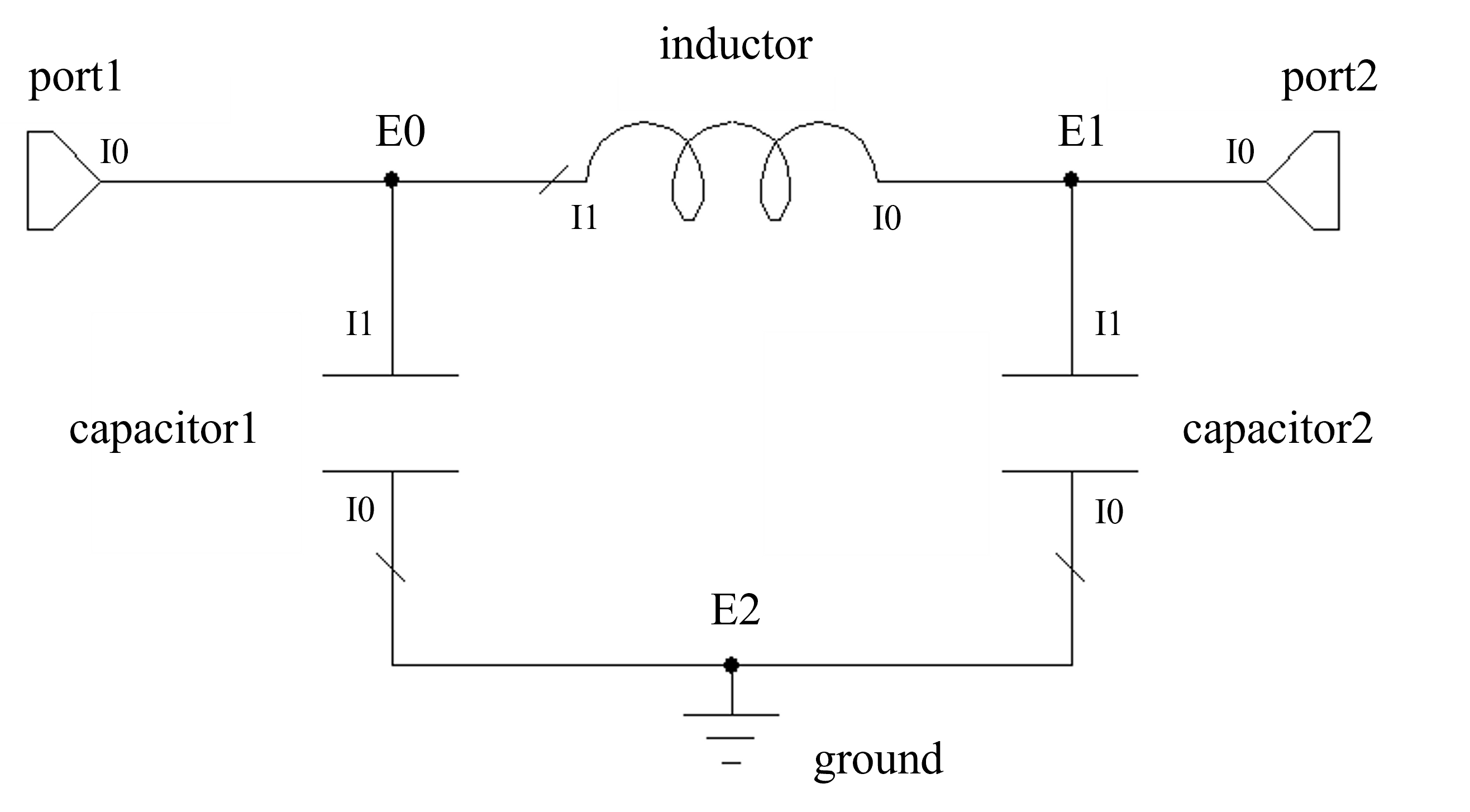
If the above sounded confusing, don’t worry - the method is easy to understand using a simple example. Below we define a two-port PI-CLC network using the Circuit class. “External” nodes (each entry in the outer list) are numbered as E0, E1 etc. whereas “internal” port indices (ports for each model in the circuit) are numbered per element as I0, I1 etc.
import pmrf as prf
from pmrf.models import Capacitor, Inductor, Circuit, Port, Ground

# Instantiate the elements, ports and grounds.
# Note that ports are exposed in our new model in the order of the list
C1, C2, L = Capacitor(C=2e-12), Capacitor(C=1.5e-12), Inductor(L=3e-9)
p0, p1, ground = Port(), Port(), Ground()

# Create the connections list
connections = [
    [(p0, 0), (C1, 1), (L, 1)],         # E0 -> port 1
    [(p1, 0), (C2, 1), (L, 0)],         # E1 -> port 2
    [(ground, 0), (C1, 0), (C2, 0)],    # E2
]

# Create the model and plot it's S21 parameter
pi_clc = Circuit(connections)
freq = prf.Frequency(1, 1000, 1001, 'MHz')
pi_clc.plot_s_db(freq, m=1, n=0)

# Note that ParamRF already provides a built in, more efficient PiCLC model
from pmrf.models import PiCLC
PiCLC(2e-12, 3e-9, 1.5e-12).plot_s_db(freq, m=1, n=0)
Parameter Manipulation
Although more detailed parameter manipulation is described in the Parax documentation, we provide a basic example here for the case of compositional model building using the previous cascade example. Note that ShuntResistor, ShuntInductor, and ShuntCapacitor are marked as “transparent” Parax models, allowing their internal parameters to be directly accessed using the model name. However, for models without this flag set, the model name acts as a prefix, with the parameter variables as the suffix.
from pmrf.models import ShuntResistor, ShuntInductor, ShuntCapacitor

# Create the RLC model from before, but provide the models with names
R = ShuntResistor(100.0, name='R')
L = ShuntInductor(2.0e-9, name='L')
C = ShuntCapacitor(1.0e-12, name='C')
rlc = R ** L ** C

# Print the named parameters
print(rlc.named_params())

# We can now manipulate the model appropriately
rlc_with_fixedC = rlc.with_fixed_params('L')
rlc_with_R200 = rlc.with_params(R=200)
Hierachical Modeling
As mentioned, for more complex models (such as equation-based ones), users can inherit directly from the Model class and override one of the network properties (such as s, a, z, or y) or the __call__ method.
Any parameters in the model should be marked with the type parax.Parameter (or collections thereof), as shown below. Any other attributes, such as other regular jnp.ndarray objects, floats, strings, bools, are not registered as part of the parameter hierachy, and will not be seen by parameter inspection methods, optimizers, or samplers.
Note that although parameters must be annotated using parax.Parameter, parameter initialization is flexible:
Parameters may be populated with a simple float value, and are automatically converted as long as only
__post_init__(and not`__init__) is overriden.Factory methods such as
parax.Uniform,parax.Normalorparax.Fixedcan be used directly inline without Python mutable object reference issues.Parameters can be instantiated using the
parax.Parameterclass constructor directly.
Equation-based Models
The following example demonstrates custom model definition by defining a capacitor from first principles. Notice how C is automatically converted to a parameter and can be used as if it were a JAX array during the computation.
import jax.numpy as jnp
import parax as prx
import pmrf as prf

# Define the capacitor
class Capacitor(prf.Model):
    C: prx.Parameter = 1.0e-12

    def s(self, freq: prf.Frequency) -> jnp.ndarray:
        w, C = freq.w, self.C
        assert isinstance(self.C, prx.Parameter)
        z0_0 = z0_1 = self.z0

        # Compute the S-parameters
        denom = 1.0 + 1j * w * C * (z0_0 + z0_1)
        s11 = (1.0 - 1j * w * C * (jnp.conj(z0_0) - z0_1) ) / denom
        s22 = (1.0 - 1j * w * C * (jnp.conj(z0_1) - z0_0) ) / denom
        s12 = s21 = (2j * w * C * (z0_0.real * z0_1.real)**0.5) / denom

        # Return an array of shape (nfreq, nports, nports)
        return jnp.array([
            [s11, s12],
            [s21, s22]
        ]).transpose(2, 0, 1)

 # Instantiate the capacitor and plot s21
 Capacitor(2.0e-12).plot_s_db(prf.Frequency(10, 100, 101, 'MHz'), m=1, n=0)
Circuit Models
For complicated models, it can be convenient to inherit from pmrf.Model while still internally building the model using cascading or via Circuit.
The following example creates a PI-CLC model once again, but using this approach.
Note that, when inheriting from Model, an explicit __init__ method is not required, and one is automatically generated for you. However, it is often still desirable to have temporary init parameters separate to your model parameters. In this case, using dataclasses.InitVar in combination with __post_init is the canonical approach. This is demonstrated below.
As a last resort, overriding __init__ is still possible, but parameters must be manually converter using the parax.Parameter constructor, and super().__init__ must explicitly be called.
from dataclasses import InitVar
from parax.parameters import Uniform
import pmrf as prf
from pmrf.models import Capacitor, Inductor, Circuit, Port, Ground
import parax as prx

class PiCLC(prf.Model):
    C1_divided_by_5: InitVar[float]

    # To be instantiated in post init
    cap1: Capacitor = prx.field(init=False)
    cap2: Capacitor = Capacitor(C=Uniform(0.0, 10.0, value=2.0, scale=1e-12))
    ind: Inductor = Inductor(L=Uniform(0.0, 10.0, value=2.0, scale=1e-12))

    def __post_init__(self, C1_divided_by_5: float):
        self.cap1 = Capacitor(C1_divided_by_5 * 5.0)

    def __call__(self) -> prf.Model:
        # Instantiate the ports and grounds
        port1, port2, ground = Port(), Port(), Ground()

        # Create the connections list. This time, capacitor1, capacitor2 and inductor are members.
        connections = [
            [(port1, 0), (self.cap1, 1), (self.ind, 1)], # E0
            [(port2, 0), (self.cap2, 1), (self.ind, 0)], # E1
            [(ground, 0), (self.cap1, 0), (self.cap2, 0)], # E2
        ]

        # Return the model
        return Circuit(connections)

model = PiCLC(C1_divided_by_5=1e-12, cap2=Capacitor(1e-12), ind=Inductor(1e-9))
assert model.cap1.C.value == 1e-12 * 5.0