Custom Composite Models

In ParamRF, models can contain other models, referred to as composite models. The following example builds on top of the custom_models example to demonstrate how to build these effectively.

Before we do this, it is useful to note the following two rules when creating custom models:

• Models are immutable. If you want to change the structure of a model given an existing one, create a method named something like .with_structure that returns a new model.

• You should never store state that can be derived. All member variables should be treated as the core “dumb data” to be passed through mathematical functions.

Defining a Multi-Stage Filter

When building composite models, it is often desirable to initialize a model based on higher-level specifications. For example, you may want to specify the number of stages of a filter or its cuttoff frequency. It is best to handle this purely as an initialization step, especially because such variables can fundamentally change the model’s structure. To demonstrate this, let’s build a multi-stage LC filter:

import math
import pmrf as prf
from pmrf.models import ShuntCapacitor, Inductor, Cascade

class NStageFilter(prf.Model):
    num_stages: prf.InitVar[int]
    fc: prf.InitVar[float]

    capacitors: list[ShuntCapacitor] = prf.field(init=False)
    inductors: list[Inductor] = prf.field(init=False)

    def __post_init__(self, num_stages: int, fc: float):
        z0 = self.z0
        c_val = 1.0 / (math.pi * fc * z0)
        l_val = z0 / (math.pi * fc)

        self.capacitors = [ShuntCapacitor(C=c_val) for _ in range(num_stages + 1)]
        self.inductors = [Inductor(L=l_val) for _ in range(num_stages)]

    def build(self) -> prf.Model:
        components = [self.capacitors[0]]
        for i in range(len(self.inductors)):
            components.append(self.inductors[i])
            components.append(self.capacitors[i + 1])
        return Cascade(components)

We override build() instead of one of the matrix methods to return the model directly. Note also how we use pmrf.InitVar and pmrf.field(). This prevents us from having to manually define an __init__ method with redundant fields, and also represents good practice for separation of configuration from state.

Evaluating the Response

Because our model overrides build, it inherits all standard matrix methods. To round off the example, let’s instantiate several filters with different numbers of stages and plot their insertion loss:

import jax.numpy as jnp
import matplotlib.pyplot as plt

band = prf.Frequency(0.1, 10, 201, 'GHz')
fc = 2.4e9

for n in [1, 3, 5]:
    filter_n = NStageFilter(num_stages=n, fc=fc)
    filter_n.plot_s_db(band, m=1, n=0, label=f'{n} Stage(s)')

plt.title('Composite Multi-Stage LC Filter Response')
plt.grid(True)

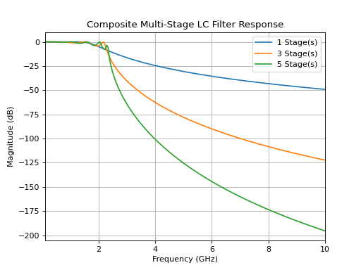
It is clear that the filter successfully starts to cut off at 2.4 GHz, and that the amount of roll-off increases as more stages are added.