Derivatives and Sweeps

ParamRF provides built-in utilities for the calculation of analytical derivatives, as well as for performing vectorized parameter and function sweeps.

Model Setup

Derivatives and sweeps can be performed across the parameters in a model. Let’s set up a base low-pass filter example model with named sub-models and unconstrained parameters, declared in pF and nH:

import pmrf as prf
from pmrf.models import ShuntCapacitor, Inductor, Cascade

c1 = ShuntCapacitor(C=prf.Unconstrained(1.0, scale=1e-12), name='c1')
l1 = Inductor(L=prf.Unconstrained(1.0, scale=1e-9), name='l1')
c2 = ShuntCapacitor(C=prf.Unconstrained(1.0, scale=1e-12), name='c2')

lpf = Cascade([c1, l1, c2])

Scalar Derivatives

To differentiate a model’s parameters, we can pass any differentiable function to pmrf.derivative() alongside its nominal arguments:

import pmrf as prf

freq = prf.Frequency(2.4, 2.4, 1, 'GHz')

def s21_mag(model):
    return model.s_mag(freq)[0,1,0]

(derivatives,) = prf.derivative(s21_mag, lpf)

sensitivities = prf.values(derivatives)

print(f"Sensitivity to C1: {sensitivities['c1.C']:.3f} / pF")
print(f"Sensitivity to L: {sensitivities['l1.L']:.3f} / nH")

Output:

Sensitivity to C1: -0.106 / pF
Sensitivity to L: 0.086 / nH

The value returned by pmrf.derivative() is a tuple with one entry per argument, each with the same structure as its argument and every parameter replaced by its derivative. We can pass in individual parameters, regular JAX arrays, or entire models (as in the above example).

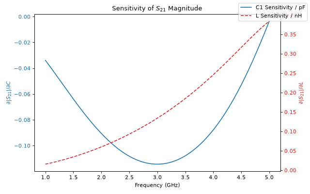
A parameter’s derivative is taken with respect to its declared value, so the sensitivities above are already per pF and per nH. Pass space='physical' for per farad and per henry, or space='raw' for the space an optimizer moves through (see Parameter Names).

Vector Jacobians

We can also evaluate derivatives/sensitivity across an entire frequency band, known as computing the jacobian:

import jax.numpy as jnp
import matplotlib.pyplot as plt

band = prf.Frequency(1, 5, 201, 'GHz')

def s21_mag_array(c1_val, l_val):
    model = (
        ShuntCapacitor(C=prf.Unconstrained(c1_val, scale=1e-12))
        ** Inductor(L=prf.Unconstrained(l_val, scale=1e-9))
        ** ShuntCapacitor(C=prf.Unconstrained(1.0, scale=1e-12))
    )
    return model.s_mag(band)[:,1,0]

c_nom, l_nom = jnp.array(1.0), jnp.array(1.0)
ds21_dc, ds21_dl = prf.derivative(s21_mag_array, c_nom, l_nom)

In the above example, we passed JAX arrays holding values in pF and nH and built the parameters inside the function, so the derivatives are per pF and per nH. We can plot the results as a function of frequency to visualize their behaviour:

fig, ax1 = plt.subplots(figsize=(8, 5))

ax1.plot(band.f_scaled, ds21_dc, color='tab:blue', label='C1 Sensitivity / pF')
ax1.set_xlabel('Frequency (GHz)')
ax1.set_ylabel(r'$\partial |S_{21}| / \partial C$', color='tab:blue')
ax1.tick_params(axis='y', labelcolor='tab:blue')

ax2 = ax1.twinx()
ax2.plot(band.f_scaled, ds21_dl, color='tab:red', linestyle='--', label='L Sensitivity / nH')
ax2.set_ylabel(r'$\partial |S_{21}| / \partial L$', color='tab:red')
ax2.tick_params(axis='y', labelcolor='tab:red')

plt.title('Sensitivity of $S_{21}$ Magnitude')
fig.legend()
fig.tight_layout()

Parallel Sweeps

We can perform vectorized sweeps using pmrf.sweep(). By default, this is done in a parallel (zip-like) manner across the leading dimension of input JAX arrays. For example, lets sweep \(C_1\) and \(L_1\) simultaneously over a 1D range of values to evaluate the filter’s insertion loss (\(S_{21}\)) at 2.4 GHz:

c_sweep = jnp.linspace(0.5, 1.5, 50)   # pF
l_sweep = jnp.linspace(0.5, 1.5, 50)   # nH

def eval_s21_mag(c_val, l_val):
    model = (
        ShuntCapacitor(C=prf.Unconstrained(c_val, scale=1e-12))
        ** Inductor(L=prf.Unconstrained(l_val, scale=1e-9))
        ** ShuntCapacitor(C=prf.Unconstrained(1.0, scale=1e-12))
    )
    return model.s_mag(freq)[0, 1, 0]

s21_parallel = prf.sweep(eval_s21_mag, c_sweep, l_sweep)
print(f"Parallel sweep output shape: {s21_parallel.shape}")

Output:

Parallel sweep output shape: (50,)

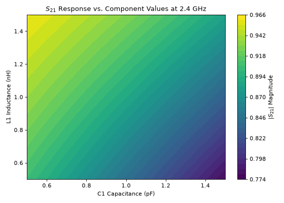
Grid Sweeps

If we instead want to evaluate the function across every possible combination of inputs, we can pass grid=True. The output will be reshaped into an N-dimensional array corresponding to the swept dimensions. Let’s use this to visualize the \(S_{21}\) magnitude as a 2D surface across our component values:

s21_grid = prf.sweep(eval_s21_mag, c_sweep, l_sweep, grid=True)

fig, ax = plt.subplots(figsize=(7, 5))

C, L = jnp.meshgrid(c_sweep, l_sweep, indexing='ij')

surface = ax.contourf(C, L, s21_grid, levels=30, cmap='viridis')
fig.colorbar(surface, ax=ax, label='$|S_{21}|$ Magnitude')

ax.set_xlabel('C1 Capacitance (pF)')
ax.set_ylabel('L1 Inductance (nH)')
plt.title('$S_{21}$ Response vs. Component Values at 2.4 GHz')
fig.tight_layout()